| info.html, history.html, glossary.html | |
|
Translate: French | German | Italian | Japanese | Spanish | Portuguese |
|
Of EconGuru |
Back to Previous Page |
Fundamentals of Ecology
Ecological Populations
| « Chapter 1 | Contents | Chapter 3 » |
2. Populations
A population is defined as all the organism within an area belonging to the same species. At this ecological level, ecologists are interested in the growth and regulation of population size, as well as the factors behind them.
2.1. Density, Distribution and Size
Population density is the number of individuals of a certain species per unit area or volume, and population distribution is the pattern of dispersal of them within that area. They both are indispensable variables for ecologists to analyze and discover the spreading pattern of a certain species within a certain area and time. Consider calculating the average density of people in the United States, but we know very well that most people live in cities where the number of people per unit area is dramatically higher than that in the country. Therefore, basing ecological population models solely on density can be misleading.
The density and distribution of a population changes with time, due to abiotic factors(inorganic factors) as well as biotic factors(organic factors). Abiotic factors that could have an influence on a population include temperature, rainfall, type of soil and so forth; biotic factors are those that are related to other living things. For example, a particular kind of plant pervading only in a particular area is very likely to affect the density and distribution of a population of an animal that feeds only on it. In these situations, limiting factors are those that particularly determine whether an organism lives in an area.
Example of a Limiting Factor
In mountainous regions and high latitudes, timberline is the limit of tree growth. Trees cannot grow above the high timberline because water remains frozen at the low temperature for most of the year. In this case, timberline, or more specifically, temperature is the limiting factor for tree density and distribution.
Population size is the number of individuals in a population. Technically, genetic relationship is used to distinguish whether an individual belongs to a population or not. Instead of simply counting for the number, it is necessary to estimate the present population size, methods of which vary with the kind of species in question.
Just as density and distribution, population size fluctuates in time. But what factors would affect the future size of a population? There are generally four sources of contribution to the fluctuation of a population size, natality(rate of birth), mortality(rate of death), immigration and emigration. How they each changes the population size is indicated below.
| Immigration | ||||
| Natality | Population Size | Mortality | ||
| Emigration |
Usually it is acceptable to assume that immigration and emigration are about equal and therefore only necessary to consider natality and mortality.
2.2. Growth Patterns
Theoretically, there exist 2 distinct and simple growth patterns, or mathematical models for population growth. In the first one, only one reproductive chance is given to members of the population during in their entire lifespan. Once mission accomplishes, they die. Many insects and annual plants reproduce in this manner. In the other model, members experience many reproductive events throughout their lifetime. Most vertebrates, and trees have this pattern of reproduction.
Expressed in mathematical equations and graphs, the 2 growth patterns can be referred as the exponential growth pattern and the logistic growth pattern respectively. We are not going to resort to number and equation here, but a glance at the graphs below will be enough for this introductory course.
Population Exponential Growth
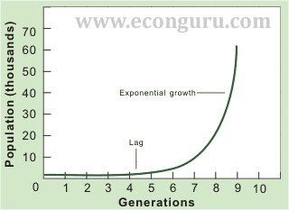
Lag phase: Growth is slow because population base is small.
Exponential growth phase: Growth is accelerating, that is, the rate of growth itself grows.
Population Logistic Growth
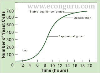
Lag phase: Growth is slow because the population base is small.
Exponential growth phase: Growth is accelerating, that is, the rate of growth itself grows.
Deceleration phase: The rate of population growth slows down.
Stable equilibrium phase: Little growth because births and deaths are about equal.
Plus, since a population is constantly being affected and shaped by its environment, biotically or abiotically, real world growth patterns are more complex and entangling.
2.3. Mortality Patterns and Survivorship Curves
Population growth patterns require an assumption that members of a population are all identical individuals. However, individuals are in their different stages of lifespan. In a given period of time, some are born and some die. See if you can figure out the data in this table:
| Age (month) |
Number Observed Alive | Proportion Surviving | Number Dying | Mortality Rate Per Capita |
Avg. Number of Seeds/Individuals |
|---|---|---|---|---|---|
| 0-3 | 843 | 1,000 | 121 | 0.143 | 0 |
| 3-6 | 722 | 857 | 195 | 0.271 | 300 |
| 6-9 | 527 | 625 | 211 | 0.400 | 620 |
| 9-12 | 316 | 375 | 172 | 0.544 | 430 |
| 12-15 | 144 | 171 | 95 | 0.626 | 210 |
| 15-18 | 54 | 64 | 39 | 0.722 | 60 |
| 18-21 | 15 | 17.8 | 12 | 0.800 | 30 |
| 21-24 | 3 | 3.6 | 3 | 1.000 | 10 |
| 24 | 0 | - | - | - | - |
A cohort of a population, is the total number of new births of it at the same time. As you can see, the number of grass observed alive at the beginning is 843, and data are noted down every 3 months. The grass are gradually dying out, and the life stages at which they perish vary. From another perspective, let's look at the number that survives instead of focusing on the number dying in each period. After the first observational period, 722 survive the first 3 months. Survivorship is the probability of newborn individuals of a cohort surviving to particular ages. Plotting the number surviving against percent of life span, we get survivorship curves that show the number of individuals of a cohort still living over time.
For the sake of discussion, we will establish three types of representative survivorship curves hypothetically, displayed in the upper left graph of the following image. Curve I is characteristic of a population in which most individuals survive well pass the midpoint. On the contrary, Curve III typifies populations wherein most individuals die young. In the type II curve, survivorship decreases at a constant rate throughout the lifespan.
Survivorship Curves
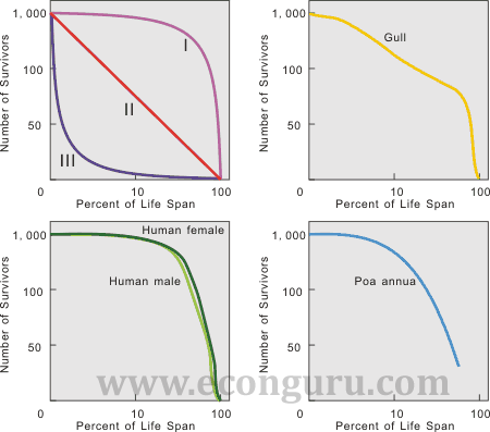
Survivorship curves denote mortality patterns of a certain population over a certain period of time. It may vary in abnormal conditions, but in most cases the pattern stay predictable.
2.4. Age Distribution
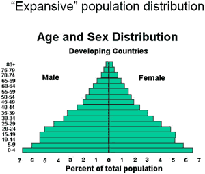
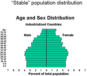
To focus on population growth, we divide a population into three major age groups, that is prereproductive, reproductive, and postreproductive. From this point of view, populations differ with respect to the proportion of each age group in the entirety. Basically, we can derive two typical age structure diagrams.
Sources: http://www.wri.org
When preproductive group is the largest of the three, as in the "expansive" age distribution, the birthrate is higher than the death rate, and a pyramid-shaped diagram is expected. Under such conditions, there are more individuals entering than leaving the reproductive years. Eventually, as the size of reproductive group equals that of prereproductive group, a bell-shaped diagram results, that is the "stable" age distribution.
Normally, the "expansive" age distribution is seen frequently in developing countries, such as African countries, while the "stable" pattern is a typical developed country pattern with a low birthrate. Nonetheless, a third pattern exists to explain a few of the shrinking populations that are present in countries like Sweden. Search the web if you are interested.
| « Chapter 1 | Contents | Chapter 3 » |
Of EconGuru |
Back to Previous Page |